Coverage Reasons
Let $f$ be a Boolean function represented by a random forest $RF$, $x$ be an instance and $1$ (resp. $0$) the prediction of $RF$ on $x$ ($f(x) = 1$ (resp. $f(x)=0$)). The Boolean conditions occurring in the trees are often logically connected: such constraints are gathered in a domain theory $\Sigma^f$ (for instance, the condition $A_1 > 30$ entails the condition $A_1 > 20$). Domain theories are described in the Theories page.
A coverage-based prime implicant explanation (CPI-Xp), or coverage reason, for $x$ is an abductive explanation for $x$ that is maximally general with respect to the domain theory $\Sigma^f$. An abductive explanation is a subset $t$ of the characteristics (Boolean conditions) of $x$ such that every instance sharing $t$ and satisfying $\Sigma^f$ is classified by $f$ in the same way as $x$ (in other words, $t$ is an implicant of $f$ modulo $\Sigma^f$). Among all the abductive explanations of $x$, a coverage reason is one that covers as many instances satisfying $\Sigma^f$ as possible: no other abductive explanation of $x$ is strictly more general modulo $\Sigma^f$.
A coverage reason is not necessarily a sufficient reason. A sufficient reason is a prime (i.e. subset-minimal) implicant of $f$ covering $x$, whereas a coverage reason is selected for its generality and not for its minimality. Because of the constraints in $\Sigma^f$, maximizing generality may require keeping many conditions, so a coverage reason can involve far more Boolean conditions than a sufficient reason (it need not be subset-minimal). What a coverage reason does guarantee is that it never retains a condition subsumed by a more general one under the theory (for example, it keeps $A_1 > 20$ rather than the less general $A_1 > 30$). A coverage reason that is in addition subset-minimal is called a minimal coverage reason (mCPI-Xp): no literal can be removed from it while it remains a valid implicant modulo $\Sigma^f$. More information can be found in the article Computing Coverage-Based Prime Implicant Explanations for Tree-Based Models.
The function ExplainerRF.coverage_reason allows computing a coverage reason. The function ExplainerRF.minimal_coverage_reason allows computing a minimal coverage reason: starting from a coverage reason, it greedily removes each literal and checks whether the remaining set is still a valid implicant modulo $\Sigma^f$, repeating until no literal can be discarded. Both functions rely on the domain theory, so the feature types must be provided when initializing the explainer (through the features_type parameter, see the Theories page); otherwise a ValueError is raised.
Feature order
Several coverage reasons may exist for a same instance. The ExplainerRF.coverage_reason function returns one of them, computed by a greedy algorithm that processes the features in a given priority order. This order can be controlled through the ordre_features parameter (a list of feature names); when it is not provided, a default order derived from the domain theory is used.
Example from Hand-Crafted Trees
For this example, we take the random forest below (Figure 1 of the article). It is built over two features: a numerical one $A_1$ (the annual income (in thousands of dollars) of a loan applicant) and a binary one $A_2$ (whether or not the applicant holds a permanent position). In PyXAI these features are named f1 and f2.
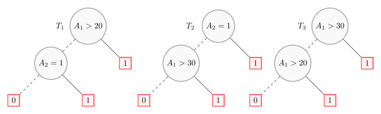
Three Boolean conditions occur in the forest: $B_1 = (A_1 > 20)$, $B_2 = (A_1 > 30)$ and $B_3 = (A_2 = 1)$. The conditions $B_1$ and $B_2$ are not independent: they are logically connected by the domain theory $\Sigma^f$ stating that $B_2 \Rightarrow B_1$ (an income above $30$ is also above $20$). Under this theory, the forest is equivalent to $f \equiv B_1 \vee B_2 \vee B_3$.
We consider the instance $x = (33, 1)$ (an applicant earning 33 thousand dollars and holding a permanent position), for which $f(x) = 1$. We start by building the forest and activating the domain theory:
from pyxai import Builder, Explaining

# T1: A1 > 20 ? 1 : (A2 = 1 ? 1 : 0)
nodeT1_A2 = Builder.DecisionNode(2, operator=Builder.EQ, threshold=1, left=0, right=1)
nodeT1_A1 = Builder.DecisionNode(1, operator=Builder.GE, threshold=20, left=nodeT1_A2, right=1)
tree1 = Builder.DecisionTree(2, nodeT1_A1)

# T2: A2 = 1 ? 1 : (A1 > 30 ? 1 : 0)
nodeT2_A1 = Builder.DecisionNode(1, operator=Builder.GE, threshold=30, left=0, right=1)
nodeT2_A2 = Builder.DecisionNode(2, operator=Builder.EQ, threshold=1, left=nodeT2_A1, right=1)
tree2 = Builder.DecisionTree(2, nodeT2_A2)

# T3: A1 > 30 ? 1 : (A1 > 20 ? 1 : 0)
nodeT3_A1_20 = Builder.DecisionNode(1, operator=Builder.GE, threshold=20, left=0, right=1)
nodeT3_A1_30 = Builder.DecisionNode(1, operator=Builder.GE, threshold=30, left=nodeT3_A1_20, right=1)
tree3 = Builder.DecisionTree(2, nodeT3_A1_30)

forest = Builder.RandomForest([tree1, tree2, tree3], n_classes=2)

instance = (33, 1)
explainer = Explaining.initialize(forest, instance=instance, features_type={"numerical": ["f1"], "binary": ["f2"]})
print("target_prediction:", explainer.target_prediction)
---------   Theory Feature Types   -----------
Before the one-hot encoding of categorical features:
Numerical features: 1
Categorical features: 0
Binary features: 1
Number of features: 2
Characteristics of categorical features: {}

Number of used features in the model (before the encoding of categorical features): 2
Number of used features in the model (after the encoding of categorical features): 2
----------------------------------------------
target_prediction: 1
For this instance, the subset-minimal abductive explanations are ${A_1 > 20}$, ${A_1 > 30}$ and ${A_2 = 1}$ (here they are also sufficient reasons, since each is a single condition). Among them, ${A_1 > 30}$ is less general than ${A_1 > 20}$ under the theory $B_2 \Rightarrow B_1$ (every instance covered by $A_1 > 30$ is also covered by $A_1 > 20$, but not the other way around). Hence the coverage reasons are only the two maximally general ones: ${A_1 > 20}$ and ${A_2 = 1}$.
We first compute a sufficient reason, then a coverage reason:
sufficient = explainer.sufficient_reason()
print("sufficient:", explainer.to_features(sufficient))

coverage = explainer.coverage_reason()
print("coverage:", explainer.to_features(coverage))
sufficient: ['f2 == 1']
coverage: ['f2 == 1']
By default the greedy algorithm returns the coverage reason ${A_2 = 1}$. Using the ordre_features parameter, we can change the priority order over the features and obtain the other coverage reason ${A_1 > 20}$:
coverage_f2_first = explainer.coverage_reason(ordre_features=["f2", "f1"])
print("coverage (f2 first):", explainer.to_features(coverage_f2_first))

coverage_f1_first = explainer.coverage_reason(ordre_features=["f1", "f2"])
print("coverage (f1 first):", explainer.to_features(coverage_f1_first))
coverage (f2 first): ['f1 >= 20']
coverage (f1 first): ['f2 == 1']
In both cases, the condition $A_1 > 30$ is never selected: a coverage reason always prefers the more general condition $A_1 > 20$.
Example from a Real Dataset
For this example, we take the australian credit approval dataset, together with the australian_0.types file describing the feature types (this file activates the domain theory; see the Theories page). We create a model using the hold-out approach and select a well-classified instance.
from pyxai import Learning, Explaining

learner = Learning.Scikitlearn("../../dataset/australian_0.csv", problem_type=Learning.CLASSIFICATION)
model = learner.evaluate(splitting_method=Learning.HOLD_OUT, model_type=Learning.RF)
instance, prediction = learner.get_instances(model, n=1, seed=11200, is_correct=True)
--------------   Information   ---------------
Problem type: classification
Instances type: tabular
Labels type: classes

Dataset path: ../../dataset/australian_0.csv
nFeatures (nAttributes, with the labels): 38
nInstances (nObservations): 690
nLabels: 2
---------------   Model creation, fitting and evaluation  ---------------
Splitting method: hold-out
Problem type: classification
Models type: random-forest
model_parameters: {}


---------   Evaluation Information   ---------
For the evaluation number 0:
Metrics:
   sklearn_confusion_matrix: [[91, 8], [11, 63]]
   precision: 88.73239436619718
   recall: 85.13513513513513
   f1_score: 86.89655172413794
   specificity: 91.91919191919192
   true_positive: 63
   true_negative: 91
   false_positive: 8
   false_negative: 11
   accuracy: 89.01734104046243
Number of Training instances: 517
Number of Testing instances: 173

---------------   Explainer   ----------------
For the split number 0:
**Random Forest Model**
nClasses: 2
nTrees: 100
nVariables: 1473

---------------   Instances   ----------------


Number of instances selected: 1
----------------------------------------------
We initialize the explainer with the domain theory and compute a coverage reason. The raw explanation is a term over the Boolean conditions of the forest (it is an implicant modulo the theory, so it may gather many literals); the to_features method gives a compact and human-readable form.
explainer = Explaining.initialize(model, instance=instance, features_type="../../dataset/australian_0.types")
print("prediction:", prediction)

coverage = explainer.coverage_reason()
print("\nlen coverage (literals):", len(coverage))
print("\ncoverage (to_features):", explainer.to_features(coverage))
---------   Theory Feature Types   -----------
Before the one-hot encoding of categorical features:
Numerical features: 6
Categorical features: 4
Binary features: 4
Number of features: 14
Characteristics of categorical features: {'A4_1': ['A4', 1, [1, 2, 3]], 'A4_2': ['A4', 2, [1, 2, 3]], 'A4_3': ['A4', 3, [1, 2, 3]], 'A5_1': ['A5', 1, [1, 2, 3, 4, 5, 6, 7, 8, 9, 10, 11, 12, 13, 14]], 'A5_2': ['A5', 2, [1, 2, 3, 4, 5, 6, 7, 8, 9, 10, 11, 12, 13, 14]], 'A5_3': ['A5', 3, [1, 2, 3, 4, 5, 6, 7, 8, 9, 10, 11, 12, 13, 14]], 'A5_4': ['A5', 4, [1, 2, 3, 4, 5, 6, 7, 8, 9, 10, 11, 12, 13, 14]], 'A5_5': ['A5', 5, [1, 2, 3, 4, 5, 6, 7, 8, 9, 10, 11, 12, 13, 14]], 'A5_6': ['A5', 6, [1, 2, 3, 4, 5, 6, 7, 8, 9, 10, 11, 12, 13, 14]], 'A5_7': ['A5', 7, [1, 2, 3, 4, 5, 6, 7, 8, 9, 10, 11, 12, 13, 14]], 'A5_8': ['A5', 8, [1, 2, 3, 4, 5, 6, 7, 8, 9, 10, 11, 12, 13, 14]], 'A5_9': ['A5', 9, [1, 2, 3, 4, 5, 6, 7, 8, 9, 10, 11, 12, 13, 14]], 'A5_10': ['A5', 10, [1, 2, 3, 4, 5, 6, 7, 8, 9, 10, 11, 12, 13, 14]], 'A5_11': ['A5', 11, [1, 2, 3, 4, 5, 6, 7, 8, 9, 10, 11, 12, 13, 14]], 'A5_12': ['A5', 12, [1, 2, 3, 4, 5, 6, 7, 8, 9, 10, 11, 12, 13, 14]], 'A5_13': ['A5', 13, [1, 2, 3, 4, 5, 6, 7, 8, 9, 10, 11, 12, 13, 14]], 'A5_14': ['A5', 14, [1, 2, 3, 4, 5, 6, 7, 8, 9, 10, 11, 12, 13, 14]], 'A6_1': ['A6', 1, [1, 2, 3, 4, 5, 7, 8, 9]], 'A6_2': ['A6', 2, [1, 2, 3, 4, 5, 7, 8, 9]], 'A6_3': ['A6', 3, [1, 2, 3, 4, 5, 7, 8, 9]], 'A6_4': ['A6', 4, [1, 2, 3, 4, 5, 7, 8, 9]], 'A6_5': ['A6', 5, [1, 2, 3, 4, 5, 7, 8, 9]], 'A6_7': ['A6', 7, [1, 2, 3, 4, 5, 7, 8, 9]], 'A6_8': ['A6', 8, [1, 2, 3, 4, 5, 7, 8, 9]], 'A6_9': ['A6', 9, [1, 2, 3, 4, 5, 7, 8, 9]], 'A12_1': ['A12', 1, [1, 2, 3]], 'A12_2': ['A12', 2, [1, 2, 3]], 'A12_3': ['A12', 3, [1, 2, 3]]}

Number of used features in the model (before the encoding of categorical features): 14
Number of used features in the model (after the encoding of categorical features): 37
----------------------------------------------
prediction: 1


len coverage (literals): 473

coverage (to_features): ['A4 = 2', 'A5 = 9', 'A6 = 4', 'A8 = 1', 'A9 = 1', 'A10 in ]4.5, 18.5]', 'A12 = 2', 'A13 in ]12.5, 33.5]', 'A14 <= 5.0']
Each categorical feature (here $A_4$, $A_5$, $A_6$ and $A_{12}$) is one-hot encoded into several binary columns, but thanks to the domain theory the explanation reports a single equality condition per categorical feature (for example A4 = 2) instead of a scattered set of literals over its binary columns. For the numerical features, the widest thresholds compatible with the prediction are kept, so that the explanation covers as many instances as possible (for example A14 <= 5.0 or A10 in ]4.5, 18.5]).
Other types of explanations are presented in the Explanations Computation page.