Quick Start
Once pyxai has been installed, you can use these commands:
python3 <file.py>: Execute a python file with lines of code using PyXAI
python3 -m pyxai -gui: Open the PyXAI’s Graphical User Interface
python3 -m pyxai -explanations: Copy the explanations backups of GUI in your current directory
python3 -m pyxai -examples: Copy the examples in your current directory
Let us give a quick illustration of PyXAI, showing how to compute explanations given an ML model. 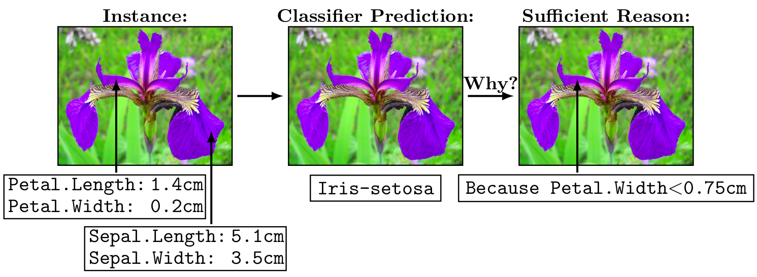
The first thing to do is to import the components of PyXAI. In order to import only the necessary methods into a project, PyXAI is composed of three distinct modules: Learning, Explaining, and Tools.
from pyxai import Learning, Explaining, Tools
If you encounter a problem, this is certainly because you need the python package PyXAI to be installed on your system. You need to execute a command like python3 -m pip install pyxai. See the Installation page for details.
In most situations, the use of PyXAI library requires two successive steps: first the generation of an ML model from a dataset (with the Learning module) and second, given the learned model, the computation of explanations for some instances (using the Explaining module).
Machine Learning
For this example, we want to create a decision tree classifier for the iris dataset using Scikit-learn.
learner = Learning.Scikitlearn("../dataset/iris.csv", problem_type='classification')
--------------   Information   ---------------
Problem type: classification
Instances type: tabular
Labels type: classes

Dataset path: ../dataset/iris.csv
nFeatures (nAttributes, with the labels): 4
nInstances (nObservations): 150
nLabels: 3
It is possible to download this dataset from the UCI Machine Learning Repository – Iris Data Set or here. In our case, it is located in the directory ../dataset. The parameter problem_type='classification' specifies a classification task. The Iris Dataset contains four features (length and width of sepals and petals) of 50 samples of three species of Iris (Iris setosa, Iris virginica and Iris versicolor). The goal of the classifier is to find the right outcome for an instance among three classes: setosa, virginica, versicolor.
To create models, PyXAI implements methods to directly run an ML experimental protocol (with the train-test split technique). Several cross-validation methods (Learning.HOLD_OUT, Learning.K_FOLDS, Learning.LEAVE_ONE_GROUP_OUT) and models (Learning.DT, Learning.RF, Learning.BT) are available.
In this example, we compute a Decision Tree (see the parameter model_type=Learning.DT).
model = learner.evaluate(splitting_method=Learning.HOLD_OUT, model_type=Learning.DT, model_parameters={'random_state': 0}, splitting_parameters={'random_state': 0})
---------------   Model creation, fitting and evaluation  ---------------
Splitting method: hold-out
Problem type: classification
Models type: decision-tree
model_parameters: {'random_state': 0}
---------   Evaluation Information   ---------
For the evaluation number 0:
Metrics:
   micro_averaging_accuracy: 98.24561403508771
   micro_averaging_precision: 97.36842105263158
   micro_averaging_recall: 97.36842105263158
   macro_averaging_accuracy: 98.24561403508773
   macro_averaging_precision: 96.66666666666667
   macro_averaging_recall: 97.91666666666666
   true_positives: {'Iris-setosa': 13, 'Iris-versicolor': 15, 'Iris-virginica': 9}
   true_negatives: {'Iris-setosa': 25, 'Iris-versicolor': 22, 'Iris-virginica': 28}
   false_positives: {'Iris-setosa': 0, 'Iris-versicolor': 0, 'Iris-virginica': 1}
   false_negatives: {'Iris-setosa': 0, 'Iris-versicolor': 1, 'Iris-virginica': 0}
   accuracy: 97.36842105263158
   sklearn_confusion_matrix: [[13, 0, 0], [0, 15, 1], [0, 0, 9]]
Number of Training instances: 112
Number of Testing instances: 38

---------------   Explainer   ----------------
For the split number 0:
**Decision Tree Model**
nFeatures: 4
nNodes: 6
nVariables: 5
Once the model is created, we select an instance in order to be able to derive explanations. Here, a well-classified instance is chosen: the model predicts the first class 0 (i.e. the Iris setosa class) thanks to the is_correct=True and the subset_predicted_classes=["Iris-setosa"] parameters.
instance, prediction = learner.get_instances(model, n=1, is_correct=True, subset_predicted_classes=["Iris-setosa"], seed=2)
---------------   Instances   ----------------
Number of instances selected: 1
----------------------------------------------
Please consult the Learning page for more details about this ML part.
Explainer
The Explainer module contains different methods to generate explanations. For this purpose, the model and the target instance are defined as parameters of the initialize function of this module.
explainer = Explaining.initialize(model, instance)
The initialize function converts the instance into binary variables (called a binary representation) coding the associated model. More precisely, each of these binary variables represents a condition (feature $op$ value ?) in the model where $op$ is a standard comparison operator. Scikit-learn and XGBoost use the operator $\ge$. With respect to the instance, the sign of a binary variable indicates whether the condition is true or not in the model. Here, we can see the instance and its binary representation. We can see the conditions related to the binary representation using the function to_features which is explained below.
print("instance:", instance)
print("binary representation:", explainer.binary_representation)
print("conditions related to the binary representation:", explainer.to_features(explainer.binary_representation,eliminate_redundant_features=False))
instance: Sepal.Length    5.0
Sepal.Width     3.3
Petal.Length    1.4
Petal.Width     0.2
Name: 49, dtype: float64
binary representation: (-1, -2, -3, 4, -5)
conditions related to the binary representation: ['Sepal.Width > 3.100000023841858', 'Petal.Length <= 4.950000047683716', 'Petal.Width <= 0.800000011920929', 'Petal.Width <= 1.6500000357627869', 'Petal.Width <= 1.75']
We notice that the binary representation of this instance contains more than 4 variables because the decision tree of the model is composed of five nodes (binary variables). Indeed, the feature Petal.Width appears 3 times whereas Sepal.Length is useless. Please see the concepts page for more information on binary representations.
It is also possible to display a more compact representation by setting eliminate_redundant_features=True (the default value), which removes redundant conditions on the same feature:
print("compact representation:", explainer.to_features(explainer.binary_representation, eliminate_redundant_features=True))
compact representation: ['Sepal.Width > 3.100000023841858', 'Petal.Length <= 4.950000047683716', 'Petal.Width <= 0.800000011920929']
Abductive explanations
In PyXAI, several types of explanation are available. In their binary forms representing conditions, these are called reasons. In our example, we choose to compute one of the most popular type of explanations: a sufficient reason. A sufficient reason is an abductive explanation (any other instance X’ sharing the conditions of this reason is classified by the model as X is) for which no proper subset of this reason is a sufficient reason (i.e., the explanation is minimal with respect to set inclusion).
sufficient_reason = explainer.sufficient_reason(n=1)
print("sufficient_reason:", sufficient_reason)
sufficient_reason: (-1,)
We can get the features involved in the reason thanks to the method to_features:
print("to_features:", explainer.to_features(sufficient_reason))
to_features: ['Petal.Width <= 0.800000011920929']
The to_features method eliminates redundant features by default and is also able to return more information about the features using the details parameter. This method is described in the concepts page.
We can check whether the derived explanation actually is a reason.
print("is sufficient: ", explainer.is_sufficient_reason(sufficient_reason))
is sufficient: True
It is important to note that computing and checking reasons are done independently.
To conclude, the sufficient reason (('Petal.Width <= 0.8',)) explains why the instance [5.0 3.3 1.4 0.2] is well classified by the model (the prediction was Iris-setosa). It is because the fourth feature (the petal width in cm), set to 0.2 cm, is less than or equal to 0.8 cm (see the attached image).
Contrastive explanations
Now, let us consider another instance, a wrongly classified one using the parameter is_correct=False of the function get_instances. We set this instance to the explainer with the set_instance method.
instance, prediction = learner.get_instances(model, n=1, is_correct=False, seed=2)
explainer.set_instance(instance)
print("The prediction: ", explainer.target_prediction)
---------------   Instances   ----------------
Number of instances selected: 1
----------------------------------------------
The prediction:  Iris-virginica
We can explain why this instance is not classified differently by providing a contrastive explanation.
contrastive_reason = explainer.contrastive_reason()
print("contrastive reason", contrastive_reason)
print("to_features:", explainer.to_features(contrastive_reason, contrastive=True))
contrastive reason (1,)
to_features: ['Petal.Width > 0.800000011920929']
print(instance)
Sepal.Length    6.0
Sepal.Width     2.7
Petal.Length    5.1
Petal.Width     1.6
Name: 83, dtype: float64
# By changing the feature Petal.Width to less than or equal to 0.8 we obtain a different classification
instance['Petal.Width'] = 0.5
print(instance)
explainer.set_instance(instance)
print("Prediction: ", explainer.target_prediction)
Sepal.Length    6.0
Sepal.Width     2.7
Petal.Length    5.1
Petal.Width     0.5
Name: 83, dtype: float64
Prediction:  Iris-setosa
More information about explanations can be found in the Explainer Principles page, the Explaining Classification page and the Explaining Regression page.