Building Boosted Trees
Classification
Building the Model
This page explains how to build a Boosted Tree with tree elements (nodes and leaves). To illustrate it, we take an example from the Computing Abductive Explanations for Boosted Trees paper.
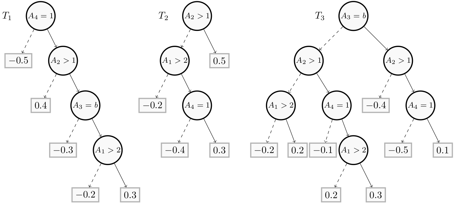
As an example of binary classification, consider four attributes: $A_1$, $A_2$ are numerical, $A_3$ is categorical, and $A_4$ is Boolean. The Boosted Tree is composed of a single forest F, which consists of three regression trees $T_1$, $T_2$, $T_3$.
First, we need to importsome modules. Let us recall that the builder module contains methods to build the Decision Tree while the explainer module provides methods to explain it.
from pyxai import Builder, Explainer, Learning
Next, we build the trees from in a bottom-up way, that is, from the leaves to the root. So we start with the $A_1 \gt 2$ node of the tree $T_1$.
node1_1 = Builder.DecisionNode(1, operator=Builder.GT, threshold=2, left=-0.2, right=0.3)
node1_2 = Builder.DecisionNode(3, operator=Builder.EQ, threshold=1, left=-0.3, right=node1_1)
node1_3 = Builder.DecisionNode(2, operator=Builder.GT, threshold=1, left=0.4, right=node1_2)
node1_4 = Builder.DecisionNode(4, operator=Builder.EQ, threshold=1, left=-0.5, right=node1_3)
tree1 = Builder.DecisionTree(4, node1_4)
We consider that the features $A_3$ and $A_4$ are numerical. Native categorical and Boolean features will be implemented in future versions of PyXAI.
Next, we build the tree $T_2$:
node2_1 = Builder.DecisionNode(4, operator=Builder.EQ, threshold=1, left=-0.4, right=0.3)
node2_2 = Builder.DecisionNode(1, operator=Builder.GT, threshold=2, left=-0.2, right=node2_1)
node2_3 = Builder.DecisionNode(2, operator=Builder.GT, threshold=1, left=node2_2, right=0.5)
tree2 = Builder.DecisionTree(4, node2_3)
And the tree $T_3$:
node3_1 = Builder.DecisionNode(1, operator=Builder.GT, threshold=2, left=0.2, right=0.3)

node3_2_1 = Builder.DecisionNode(1, operator=Builder.GT, threshold=2, left=-0.2, right=0.2)

node3_2_2 = Builder.DecisionNode(4, operator=Builder.EQ, threshold=1, left=-0.1, right=node3_1)
node3_2_3 = Builder.DecisionNode(4, operator=Builder.EQ, threshold=1, left=-0.5, right=0.1)

node3_3_1 = Builder.DecisionNode(2, operator=Builder.GT, threshold=1, left=node3_2_1, right=node3_2_2)
node3_3_2 = Builder.DecisionNode(2, operator=Builder.GT, threshold=1, left=-0.4, right=node3_2_3)

node3_4 = Builder.DecisionNode(3, operator=Builder.EQ, threshold=1, left=node3_3_1, right=node3_3_2)

tree3 = Builder.DecisionTree(4, node3_4)
We can now define the Boosted Tree:
BTs = Builder.BoostedTrees([tree1, tree2, tree3], n_classes=2)
More details about the DecisionNode and BoostedTree classes are given in the Building Models page.
Explaining the Model
Let us compute explanations. We take the same instance as in the paper, namely, ($A_1=4$, $A_2 = 3$, $A_3 = 1$, $A_4 = 1$):
instance = (4,3,1,1)

explainer = Explainer.initialize(BTs, instance)

print("target_prediction:",explainer.target_prediction)
print("binary_representation:", explainer.binary_representation)
print("to_features:", explainer.to_features(explainer.binary_representation))
target_prediction: 1
binary_representation: (1, 2, 3, 4)
to_features: ('f1 > 2', 'f2 > 1', 'f3 == 1', 'f4 == 1')
We can see that the values of binary variables are not the same as feature identifiers. Indeed, by default, binary variables have random values depending on the order with the tree is traversed. Therefore the binary variable $1$ (resp. $2$, $3$ and $4$) of this binary representation represents the condition $A_4 = 1$ (resp. $A_2 > 1$, $A_3 = 1$ and $A_1=4$).
We compute the direct reason:
direct = explainer.direct_reason()
print("direct reason:", direct)
direct_features = explainer.to_features(direct)
print("to_features:", direct_features)
assert direct_features == ('f1 > 2', 'f2 > 1', 'f3 == 1', 'f4 == 1'), "The direct reason is not correct."
direct reason: (1, 2, 3, 4)
to_features: ('f1 > 2', 'f2 > 1', 'f3 == 1', 'f4 == 1')
Now we compute a tree-specific reason:
tree_specific = explainer.tree_specific_reason()
print("tree specific reason:", tree_specific)
tree_specific_feature = explainer.to_features(tree_specific)
print("to_features:", tree_specific_feature)
print("is_tree_specific:", explainer.is_tree_specific_reason(tree_specific))
print("is_sufficient_reason:", explainer.is_sufficient_reason(tree_specific))
tree specific reason: (1, 2)
to_features: ('f2 > 1', 'f4 == 1')
is_tree_specific: True
is_sufficient_reason: True
And now we check that the reason ($A_1 = 4$, $A_4 = 1$) is a sufficient reason but not a tree-specific explanation:
reason = (1, 4)
features = explainer.to_features(reason)
print("features:", features)
print("is_sufficient_reason:", explainer.is_sufficient_reason(reason))
print("is_tree_specific:", explainer.is_tree_specific_reason(reason))
features: ('f1 > 2', 'f4 == 1')
is_sufficient_reason: True
is_tree_specific: False
The given reason consists of binary variables. Here, the binary variable $1$ (resp. $4$) represents the condition $A_4 = 1$ (resp. $A_1 = 4$ that is $A_1 > 2$).
Details on explanations are given in the Explanations Computation page.
Regression
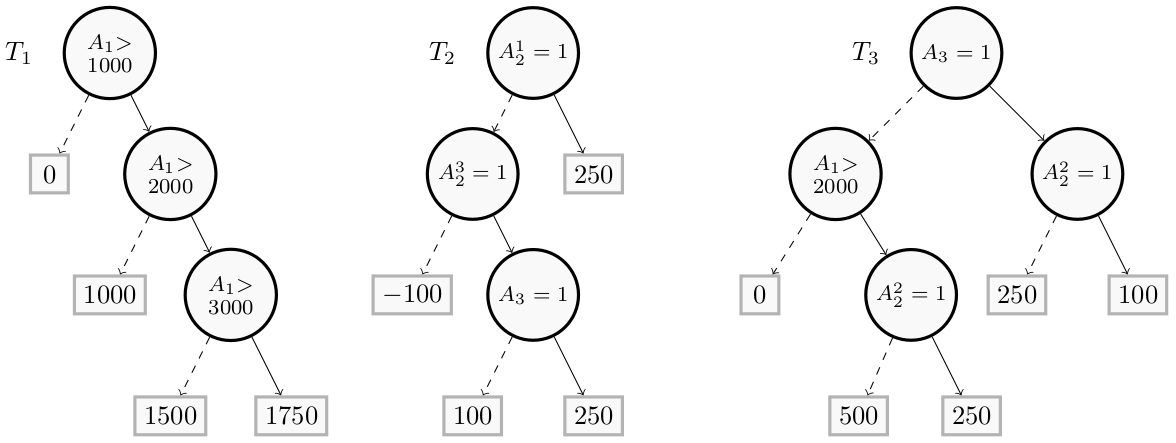
We take an example from the Computing Abductive Explanations for Boosted Regression Trees paper.
Let us consider a loan application scenario. The goal is to predict the amount of money that can be granted to an applicant described using three attributes $A = ({A_1, A_2, A_3}$).
- $A_1$ is a numerical attribute giving the income per month of the applicant
- $A_2$ is a categorical feature giving its employment status as ”employed”, ”unemployed” or ”self-employed”
- $A_3$ is a Boolean feature set to true if the customer is married, false otherwise.
In this example:
- $A_1$ is represented by the feature identifier $F_1$
- $A_2$ has been one-hot encoded and is represented by feature identifiers $F_2$, $F_3$ and $F_4$, each of these features represents respectively the conditions $A_2 = employed$, $A_2 = unemployed$ and $A_2 = self-employed$
- $A_3$ is represented by the feature identifier $F_5$ and the condition $(A_3 = 1)$ (”the applicant is married”)
Building the Model
The process is the same as for classification, except for the the last instruction that constructs the model:
BTs = Builder.BoostedTreesRegression([tree1, tree2, tree3])
has to be used for creating the model. Here is the complete procedure:
from pyxai import Builder, Explainer, Learning

node1_1 = Builder.DecisionNode(1, operator=Builder.GT, threshold=3000, left=1500, right=1750)
node1_2 = Builder.DecisionNode(1, operator=Builder.GT, threshold=2000, left=1000, right=node1_1)
node1_3 = Builder.DecisionNode(1, operator=Builder.GT, threshold=1000, left=0, right=node1_2)
tree1 = Builder.DecisionTree(5, node1_3)


node2_1 = Builder.DecisionNode(5, operator=Builder.EQ, threshold=1, left=100, right=250)
node2_2 = Builder.DecisionNode(4, operator=Builder.EQ, threshold=1, left=-100, right=node2_1)
node2_3 = Builder.DecisionNode(2, operator=Builder.EQ, threshold=1, left=node2_2, right=250)
tree2 = Builder.DecisionTree(5, node2_3)

node3_1 = Builder.DecisionNode(3, operator=Builder.EQ, threshold=1, left=500, right=250)
node3_2 = Builder.DecisionNode(3, operator=Builder.EQ, threshold=1, left=250, right=100)
node3_3 = Builder.DecisionNode(1, operator=Builder.GT, threshold=2000, left=0, right=node3_1)
node3_4 = Builder.DecisionNode(4, operator=Builder.EQ, threshold=1, left=node3_3, right=node3_2)
tree3 = Builder.DecisionTree(5, node3_4)


BTs = Builder.BoostedTreesRegression([tree1, tree2, tree3])
More details about the DecisionNode and BoostedTreesRegression classes are given in the Building Models page.
Explaining the Model
We can then compute explanations. We take the same instance as in the paper, namely,
$(2200, 0, 0, 1, 1)$ for ($F_1=2200$, $F_2 = 0$, $F_3 = 0$, $F_4 = 1$, $F_4 = 1$).
In addition, we have chosen to take a theory into account, the line "categorical": {"f{2,3,4}": (1, 2, 3)} means that the features $F_2$, $F_3$ and $F_4$ are in fact a single feature named $F{2,3,4}$ (representing $A_2$) that can take the value $1$, $2$ or $3$ (for, respectively, $A_2 = employed$, $A_2 = unemployed$ and $A_2 = self-employed$).
instance = (2200, 0, 0, 1, 1) # 2200$, self employed (one hot encoded), married
print("instance:", instance)

loan_types = {
    "numerical": Learning.DEFAULT,
    "categorical": {"f{2,3,4}": (1, 2, 3)},
    "binary": ["f5"],
}

explainer = Explainer.initialize(BTs, instance, features_type=loan_types)

print("prediction:", explainer.predict(instance))
print("condition direct:", explainer.direct_reason())
print("direct:", explainer.to_features(explainer.direct_reason()))
instance: (2200, 0, 0, 1, 1)
---------   Theory Feature Types   -----------
Before the encoding (without one hot encoded features), we have:
Numerical features: 1
Categorical features: 1
Binary features: 1
Number of features: 3
Values of categorical features: {'f2': ['f{2,3,4}', 1, (1, 2, 3)], 'f3': ['f{2,3,4}', 2, (1, 2, 3)], 'f4': ['f{2,3,4}', 3, (1, 2, 3)]}

Number of used features in the model (before the encoding): 3
Number of used features in the model (after the encoding): 5
----------------------------------------------
prediction: 2000
condition direct: (1, 2, -3, -4, 5, 6, -7)
direct: ('f1 in ]2000, 3000]', 'f{2,3,4} = 3', 'f5 == 1')
Here, with this instance ($2200$, ”self-employed”, 1), the regression value is $F(x) = 1500 + 250 + 250 = 2000$. The direct reason can also be represented by ${A_1{>}2000, \overline{A_1{>}3000}, A_2^3, A_3}$.
explainer.set_interval(1500, 2500)

tree_specific = explainer.tree_specific_reason()
print("tree specific:", explainer.to_features(tree_specific))
print("is tree : ", explainer.is_tree_specific_reason(tree_specific))
tree specific: ('f1 > 2000',)
is tree :  True
We can display this reason thank to the PyXAI GUI with:
explainer.show()

Details on explanations with regression models are given in the Explaining Regression page.