Visualization of Explanations (With GUI)
Some datasets are associated with graphical representations. It is for instance the case for the MNIST dataset (Modified National Institute of Standards and Technology database) which is a large collection of handwritten digits. Based on on PyQT6 and Matplotlib, PyXAI provides a Graphical User Interface (GUI) to display, save and load, instances and explanations for any dataset in a smart way.
You can open the PyXAI’s Graphical User Interface (GUI) with this command:
python3 -m pyxai -gui
You can also open the PyXAI’s Graphical User Interface inside a Python file thanks to the Explainer module:
from pyxai import Explainer
Explainer.show()
PyXAI saves and loads visualizations of instances and explanations through JSON files with the .explainer extension. In order to get demonstration backup files, in your current directory, we invite you to type this command:
python3 -m pyxai -explanations
This command creates a new directory containing backup files and named explanations in your current directory:
Python version:  3.10.12
PyXAI version:  1.0.post1
PyXAI location:  /home/adminlocal/Bureau/pyxai/pyxai-backend-experimental/pyxai
Source of files found:  /home/adminlocal/Bureau/pyxai/pyxai-backend-experimental/pyxai/explanations/
Successful creation of the /home/adminlocal/Bureau/pyxai/pyxai-website/explanations/ directory containing the explanations.
Loading
Open the PyXAI’s Graphical User Interface (GUI) with this command:
python3 -m pyxai -gui
Click on File and then Load Explainer in the menu bar at the top left of the application:
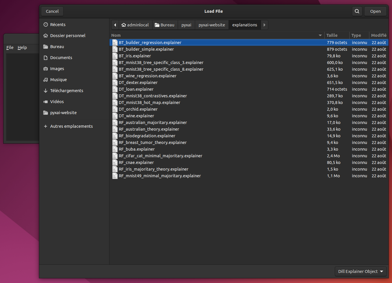
Then, you can choose the file to load, here we have chosen the file BT-iris.explainer:
Saving (with a tabular dataset)
The Australian Credit Approval dataset is a credit card application:
from pyxai import Learning, Explainer

# Machine learning part
learner = Learning.Scikitlearn("../dataset/australian_0.csv", learner_type=Learning.CLASSIFICATION)
model = learner.evaluate(method=Learning.HOLD_OUT, output=Learning.RF)
instances = learner.get_instances(model, n=10, seed=11200, correct=True)

australian_types = {
    "numerical": Learning.DEFAULT,
    "categorical": {"A4*": (1, 2, 3),
                    "A5*": tuple(range(1, 15)),
                    "A6*": (1, 2, 3, 4, 5, 7, 8, 9),
                    "A12*": tuple(range(1, 4))},
    "binary": ["A1", "A8", "A9", "A11"],
}
data:
     A1   A2   A3  A4_1  A4_2  A4_3  A5_1  A5_2  A5_3  A5_4  ...  A8  A9  A10
0     1   65  168     0     1     0     0     0     0     1  ...   0   0    1  \
1     0   72  123     0     1     0     0     0     0     0  ...   0   0    1
2     0  142   52     1     0     0     0     0     0     1  ...   0   0    1
3     0   60  169     1     0     0     0     0     0     0  ...   1   1   12
4     1   44  134     0     1     0     0     0     0     0  ...   1   1   15
..   ..  ...  ...   ...   ...   ...   ...   ...   ...   ...  ...  ..  ..  ...
685   1  163  160     0     1     0     0     0     0     0  ...   1   0    1
686   1   49   14     0     1     0     0     0     0     0  ...   0   0    1
687   0   32  145     0     1     0     0     0     0     0  ...   1   0    1
688   0  122  193     0     1     0     0     0     0     0  ...   1   1    2
689   1  245    2     0     1     0     0     0     0     0  ...   0   1    2

     A11  A12_1  A12_2  A12_3  A13  A14  A15
0      1      0      1      0   32  161    0
1      0      0      1      0   53    1    0
2      1      0      1      0   98    1    0
3      1      0      1      0    1    1    1
4      0      0      1      0   18   68    1
..   ...    ...    ...    ...  ...  ...  ...
685    0      0      1      0    1    1    1
686    0      0      1      0    1   35    0
687    0      0      1      0   32    1    1
688    0      0      1      0   38   12    1
689    0      1      0      0  159    1    1

[690 rows x 39 columns]
--------------   Information   ---------------
Dataset name: ../dataset/australian_0.csv
nFeatures (nAttributes, with the labels): 39
nInstances (nObservations): 690
nLabels: 2
---------------   Evaluation   ---------------
method: HoldOut
output: RF
learner_type: Classification
learner_options: {'max_depth': None, 'random_state': 0}
---------   Evaluation Information   ---------
For the evaluation number 0:
metrics:
   accuracy: 85.5072463768116
nTraining instances: 483
nTest instances: 207

---------------   Explainer   ----------------
For the evaluation number 0:
**Random Forest Model**
nClasses: 2
nTrees: 100
nVariables: 1361

---------------   Instances   ----------------
number of instances selected: 10
----------------------------------------------
We choose here to compute one majoritary reason per instance:
explainer = Explainer.initialize(model, features_type=australian_types)
for (instance, prediction) in instances:
    explainer.set_instance(instance)

    majoritary_reason = explainer.majoritary_reason(time_limit=10)
    print("majoritary_reason", len(majoritary_reason))
---------   Theory Feature Types   -----------
Before the encoding (without one hot encoded features), we have:
Numerical features: 6
Categorical features: 4
Binary features: 4
Number of features: 14
Values of categorical features: {'A4_1': ['A4', 1, (1, 2, 3)], 'A4_2': ['A4', 2, (1, 2, 3)], 'A4_3': ['A4', 3, (1, 2, 3)], 'A5_1': ['A5', 1, (1, 2, 3, 4, 5, 6, 7, 8, 9, 10, 11, 12, 13, 14)], 'A5_2': ['A5', 2, (1, 2, 3, 4, 5, 6, 7, 8, 9, 10, 11, 12, 13, 14)], 'A5_3': ['A5', 3, (1, 2, 3, 4, 5, 6, 7, 8, 9, 10, 11, 12, 13, 14)], 'A5_4': ['A5', 4, (1, 2, 3, 4, 5, 6, 7, 8, 9, 10, 11, 12, 13, 14)], 'A5_5': ['A5', 5, (1, 2, 3, 4, 5, 6, 7, 8, 9, 10, 11, 12, 13, 14)], 'A5_6': ['A5', 6, (1, 2, 3, 4, 5, 6, 7, 8, 9, 10, 11, 12, 13, 14)], 'A5_7': ['A5', 7, (1, 2, 3, 4, 5, 6, 7, 8, 9, 10, 11, 12, 13, 14)], 'A5_8': ['A5', 8, (1, 2, 3, 4, 5, 6, 7, 8, 9, 10, 11, 12, 13, 14)], 'A5_9': ['A5', 9, (1, 2, 3, 4, 5, 6, 7, 8, 9, 10, 11, 12, 13, 14)], 'A5_10': ['A5', 10, (1, 2, 3, 4, 5, 6, 7, 8, 9, 10, 11, 12, 13, 14)], 'A5_11': ['A5', 11, (1, 2, 3, 4, 5, 6, 7, 8, 9, 10, 11, 12, 13, 14)], 'A5_12': ['A5', 12, (1, 2, 3, 4, 5, 6, 7, 8, 9, 10, 11, 12, 13, 14)], 'A5_13': ['A5', 13, (1, 2, 3, 4, 5, 6, 7, 8, 9, 10, 11, 12, 13, 14)], 'A5_14': ['A5', 14, (1, 2, 3, 4, 5, 6, 7, 8, 9, 10, 11, 12, 13, 14)], 'A6_1': ['A6', 1, (1, 2, 3, 4, 5, 7, 8, 9)], 'A6_2': ['A6', 2, (1, 2, 3, 4, 5, 7, 8, 9)], 'A6_3': ['A6', 3, (1, 2, 3, 4, 5, 7, 8, 9)], 'A6_4': ['A6', 4, (1, 2, 3, 4, 5, 7, 8, 9)], 'A6_5': ['A6', 5, (1, 2, 3, 4, 5, 7, 8, 9)], 'A6_7': ['A6', 7, (1, 2, 3, 4, 5, 7, 8, 9)], 'A6_8': ['A6', 8, (1, 2, 3, 4, 5, 7, 8, 9)], 'A6_9': ['A6', 9, (1, 2, 3, 4, 5, 7, 8, 9)], 'A12_1': ['A12', 1, (1, 2, 3)], 'A12_2': ['A12', 2, (1, 2, 3)], 'A12_3': ['A12', 3, (1, 2, 3)]}

Number of used features in the model (before the encoding): 14
Number of used features in the model (after the encoding): 38
----------------------------------------------
majoritary_reason 12
majoritary_reason 13
majoritary_reason 12
majoritary_reason 12
majoritary_reason 13
majoritary_reason 15
majoritary_reason 13
majoritary_reason 14
majoritary_reason 13
majoritary_reason 12
And we start the PyXAI’s Graphical User Interface inside a Python file thanks to the Explainer module:
explainer.show()
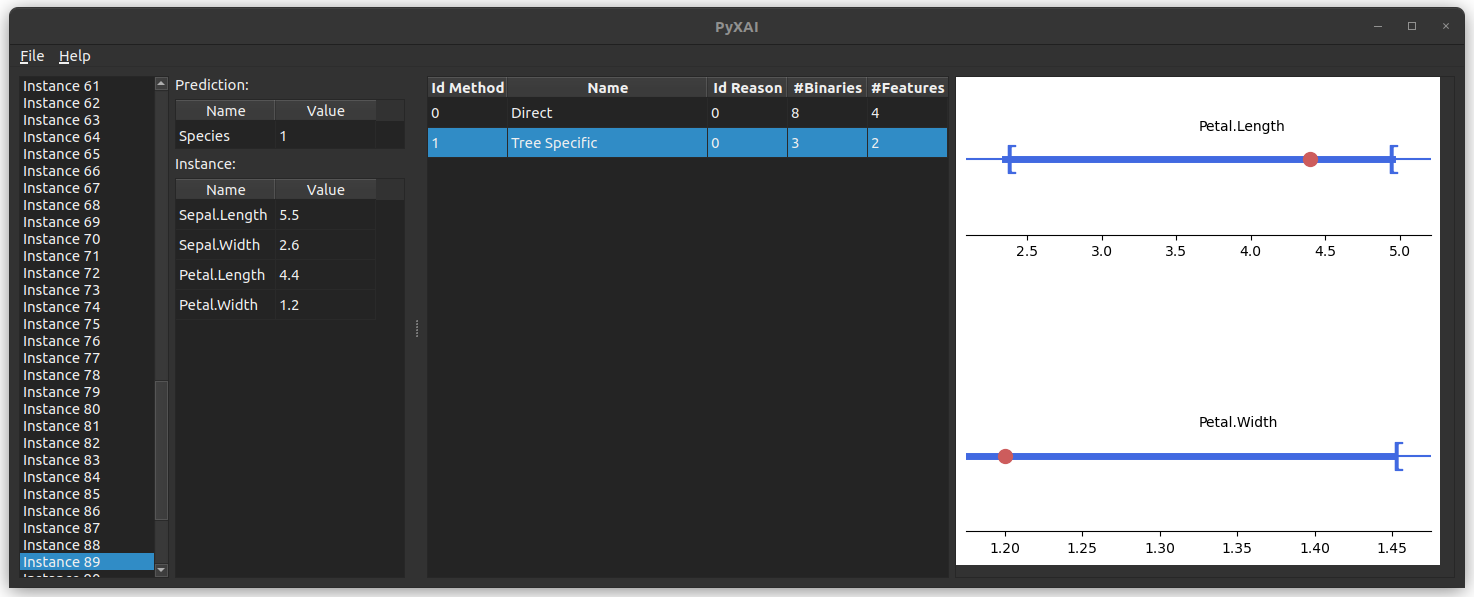
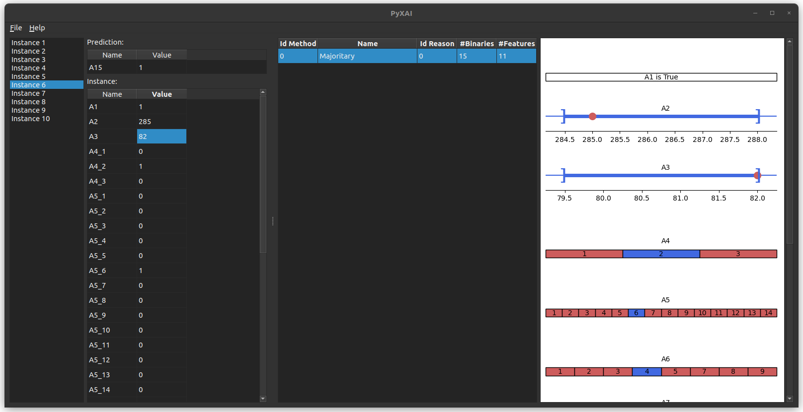
The last lines of code display the instances and the explanations:
You can save this explainer by clicking on File and then Save Explainer in the menu bar at the top left of the application.
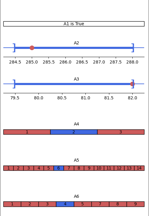
For a tabular dataset where a Theory is taken into account, an explanation is displayed according to its type:
- For Boolean features: it is indicated directly “is True” or “is False” (A_1 in the exemple)
- For categorical features: the blue (resp. red) values must be equal (resp. not equal) to explain the classification or the regression (A_4, A_5 and A_6 in the example).
- For numerical features: a horizontal axis represents the interval in which the values must be contained to explain the classification or the regression (in blue). In addition, the red dot represents the current feature value of the instance (A_2 and A_3 in the example).
Saving (with an image dataset)
We use a modified version of MNIST dataset that focuses on 4 and 9 digits. We create a model using the hold-out approach (by default, the test size is set to 30%). We choose to use a Boosted Tree by using XGBoost.
from pyxai import Learning, Explainer, Tools


# Machine learning part
learner = Learning.Xgboost("../dataset/mnist49.csv", learner_type=Learning.CLASSIFICATION)
model = learner.evaluate(method=Learning.HOLD_OUT, output=Learning.BT)
instances = learner.get_instances(model, n=10, correct=True, predictions=[0])
data:
       0  1  2  3  4  5  6  7  8  9  ...  775  776  777  778  779  780  781
0      0  0  0  0  0  0  0  0  0  0  ...    0    0    0    0    0    0    0  \
1      0  0  0  0  0  0  0  0  0  0  ...    0    0    0    0    0    0    0
2      0  0  0  0  0  0  0  0  0  0  ...    0    0    0    0    0    0    0
3      0  0  0  0  0  0  0  0  0  0  ...    0    0    0    0    0    0    0
4      0  0  0  0  0  0  0  0  0  0  ...    0    0    0    0    0    0    0
...   .. .. .. .. .. .. .. .. .. ..  ...  ...  ...  ...  ...  ...  ...  ...
13777  0  0  0  0  0  0  0  0  0  0  ...    0    0    0    0    0    0    0
13778  0  0  0  0  0  0  0  0  0  0  ...    0    0    0    0    0    0    0
13779  0  0  0  0  0  0  0  0  0  0  ...    0    0    0    0    0    0    0
13780  0  0  0  0  0  0  0  0  0  0  ...    0    0    0    0    0    0    0
13781  0  0  0  0  0  0  0  0  0  0  ...    0    0    0    0    0    0    0

       782  783  784
0        0    0    4
1        0    0    9
2        0    0    4
3        0    0    9
4        0    0    4
...    ...  ...  ...
13777    0    0    4
13778    0    0    4
13779    0    0    4
13780    0    0    9
13781    0    0    4

[13782 rows x 785 columns]
--------------   Information   ---------------
Dataset name: ../dataset/mnist49.csv
nFeatures (nAttributes, with the labels): 785
nInstances (nObservations): 13782
nLabels: 2
---------------   Evaluation   ---------------
method: HoldOut
output: BT
learner_type: Classification
learner_options: {'seed': 0, 'max_depth': None, 'eval_metric': 'mlogloss'}
---------   Evaluation Information   ---------
For the evaluation number 0:
metrics:
   accuracy: 98.57315598548972
nTraining instances: 9647
nTest instances: 4135

---------------   Explainer   ----------------
For the evaluation number 0:
**Boosted Tree model**
NClasses: 2
nTrees: 100
nVariables: 1590

---------------   Instances   ----------------
number of instances selected: 10
----------------------------------------------
# Explanation part
explainer = Explainer.initialize(model)
for (instance, prediction) in instances:
    explainer.set_instance(instance)

    direct = explainer.direct_reason()
    print("len direct:", len(direct))

    tree_specific_reason = explainer.tree_specific_reason()
    print("len tree_specific_reason:", len(tree_specific_reason))

    minimal_tree_specific_reason = explainer.minimal_tree_specific_reason(time_limit=100)
    print("len minimal tree_specific_reason:", len(minimal_tree_specific_reason))
len direct: 335
len direct: 349
len direct: 342
len direct: 388
len direct: 348
len direct: 347
len direct: 291
len direct: 357
len direct: 346
len direct: 355
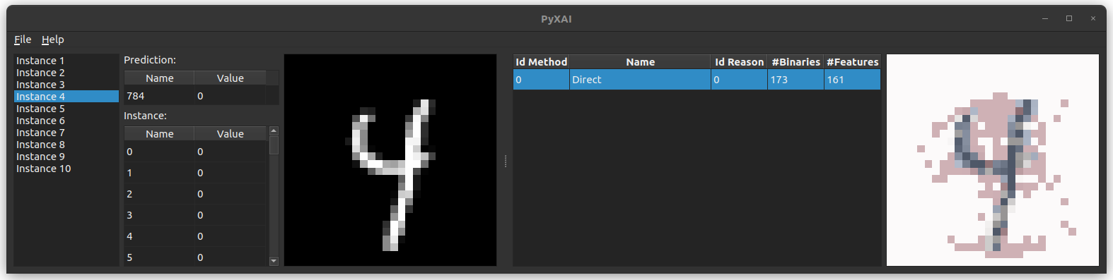
For a dataset containing images, you need to give certain information specific to images (through the image parameter of the show method) in order to display instances and explanations correctly.
| Explainer.visualisation.gui(image=None, time_series=None): |
|---|
| Open the PyXAI’s Graphical User Interface. |
image Dict None: Python dictionary containing some information specific to images with 4 keys: [“shape”, “dtype”, “get_pixel_value”, “instance_index_to_pixel_position”]. |
| “shape”: Tuple representing the number of horizontal and vertical pixels. If the number of values representing a pixel is not equal to 1, this number must be placed is the last value of this tuple. |
| “dtype”: Domain of values for each pixel (a numpy dtype or can be a tuple of numpy dtype (for a RGB pixel for example)). |
| “get_pixel_value”: Python function with 4 parameters which returns the value of a pixel according to a pixel position (x,y). |
| “instance_index_to_pixel_position”: Python function with 2 parameters which returns a pixel position (x,y) according to an index of the instance. |
time_series Dict None: To display time series. Python dictionary where a key is the name of a time serie and each value of a key is a list containing time series feature names. |
Here we give an example for the MNIST images, each of which is composed of 28 $\times$ 28 pixels, and the value of a pixel is an 8-bit integer:
import numpy

def get_pixel_value(instance, x, y, shape):
    index = x * shape[0] + y
    return instance[index]

def instance_index_to_pixel_position(i, shape):
    return i // shape[0], i % shape[0]

explainer.visualisation.gui(image={"shape": (28,28),
                      "dtype": numpy.uint8,
                      "get_pixel_value": get_pixel_value,
                      "instance_index_to_pixel_position": instance_index_to_pixel_position})
You can save this explainer by clicking on File and then Save Explainer in the menu bar at the top left of the application.
As an example, we also consider images in dataset CIFAR, which are 32 x 32 pixels with three 8-bit values (RGB) per pixel:
def get_pixel_value(instance, x, y, shape):
    n_pixels = shape[0]*shape[1]
    index = x * shape[0] + y
    return (instance[0:n_pixels][index], instance[n_pixels:n_pixels*2][index],instance[n_pixels*2:][index])

def instance_index_to_pixel_position(i, shape):
    n_pixels = shape[0]*shape[1]
    if i < n_pixels:
        value = i
    elif i >= n_pixels and i < n_pixels*2:
        value = i - n_pixels
    else:
        value = i - (n_pixels*2)
    return value // shape[0], value % shape[0]

explainer.visualisation.gui(image={"shape": (32,32,3),
                      "dtype": numpy.uint8,
                      "get_pixel_value": get_pixel_value,
                      "instance_index_to_pixel_position": instance_index_to_pixel_position})
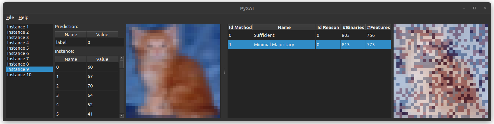
You can save individual images by clicking on File in the menu bar at the top left of the application.