PyXAI

Visualization of Explanations (Without GUI)

You can also display some explanations without the PyXAI’s Graphical Interface. To achieve this, the Explainer object of PyXAI defines several methods. As a reminder, see the Explainer page for instructions on how to create this object.

To display an explanation in a Jupyter notebook:

Explainer.visualisation.notebook(instance, reason, image=None, time_series=None, contrastive=False, width=250):
Use the `IPython.display()` method to display images in a Jupyter notebook. Displays for an instance given in the instance parameter an explanation given in the reason parameter. The given instance must be without the label. The given reason must be in Boolean variable form (without using the `to_features()` method). The explanation can be shown differently for images and time series, using the parameters provided.
instance `Numpy Array` of `Float`: The instance to be explained.
reason `List` `Tuple`: A set of (signed) binary variables. Reason (explanation) to display.
image `Dict` `None`: Python dictionary containing some information specific to images with 4 keys: [“shape”, “dtype”, “get_pixel_value”, “instance_index_to_pixel_position”].
“shape”: Tuple representing the number of horizontal and vertical pixels. If the number of values representing a pixel is not equal to 1, the last value of this tuple have to contain this number (example: (8,8,3) represents an image of 8 * 8 = 64 pixels where each pixel contains 3 values (RGB)).
“dtype”: Domain of values for each pixel (a numpy dtype or can be a tuple of numpy dtype (for a RGB pixel for example)).
“get_pixel_value”: Python function with 4 parameters which returns the value of a pixel according to a pixel position (x,y).
“instance_index_to_pixel_position”: Python function with 2 parameters which returns a pixel position (x,y) according to an index of the instance.
time_series `Dict` `None`: To display time series. Python dictionary where a key is the name of a time serie and each value of a key is a list containing time series feature names.
contrastive `Boolean`: `True` or `False` depending on whether you want to get a contrastive explanation or not. When this parameter is set to `True`, the elimination of redundant features must be reversed. Default value is `False`.
width `Integer`: The width parameter specifies width in pixels of the resulting image. Default value is `250` pixels. The width value causes the image height to be scaled in proportion to the requested width (preserves the ratio).

To display an explanation on screen:

Explainer.visualisation.screen(instance, reason, image=None, time_series=None, contrastive=False, width=250):
Use the `Image.show()` method to display images on screen with the PIL library. Displays for an instance given in the instance parameter an explanation given in the reason parameter. The given instance must be without the label. The given reason must be in Boolean variable form (without using the `to_features()` method). The explanation can be shown differently for images and time series, using the parameters provided.
instance `Numpy Array` of `Float`: The instance to be explained.
reason `List` `Tuple`: A set of (signed) binary variables. Reason (explanation) to display.
image `Dict` `None`: Python dictionary containing some information specific to images with 4 keys: [“shape”, “dtype”, “get_pixel_value”, “instance_index_to_pixel_position”].
“shape”: Tuple representing the number of horizontal and vertical pixels. If the number of values representing a pixel is not equal to 1, the last value of this tuple have to contain this number (example: (8,8,3) represents an image of 8 * 8 = 64 pixels where each pixel contains 3 values (RGB)).
“dtype”: Domain of values for each pixel (a numpy dtype or can be a tuple of numpy dtype (for a RGB pixel for example)).
“get_pixel_value”: Python function with 4 parameters which returns the value of a pixel according to a pixel position (x,y).
“instance_index_to_pixel_position”: Python function with 2 parameters which returns a pixel position (x,y) according to an index of the instance.
time_series `Dict` `None`: To display time series. Python dictionary where a key is the name of a time serie and each value of a key is a list containing time series feature names.
contrastive `Boolean`: `True` or `False` depending on whether you want to get a contrastive explanation or not. When this parameter is set to `True`, the elimination of redundant features must be reversed. Default value is `False`.
width `Integer`: The width parameter specifies width in pixels of the resulting image. Default value is `250` pixels. The width value causes the image height to be scaled in proportion to the requested width (preserves the ratio).

To return PIL images of an explanation:

Explainer.visualisation.get_PILImage(instance, reason, image=None, time_series=None, contrastive=False, width=250):
Return PIL images of the PIL library for an instance given in the instance parameter an explanation given in the reason parameter. The given instance must be without the label. The given reason must be in Boolean variable form (without using the `to_features()` method). The explanation can be shown differently for images and time series, using the parameters provided.
instance `Numpy Array` of `Float`: The instance to be explained.
reason `List` `Tuple`: A set of (signed) binary variables. Reason (explanation) to display.
image `Dict` `None`: Python dictionary containing some information specific to images with 4 keys: [“shape”, “dtype”, “get_pixel_value”, “instance_index_to_pixel_position”].
“shape”: Tuple representing the number of horizontal and vertical pixels. If the number of values representing a pixel is not equal to 1, the last value of this tuple have to contain this number (example: (8,8,3) represents an image of 8 * 8 = 64 pixels where each pixel contains 3 values (RGB)).
“dtype”: Domain of values for each pixel (a numpy dtype or can be a tuple of numpy dtype (for a RGB pixel for example)).
“get_pixel_value”: Python function with 4 parameters which returns the value of a pixel according to a pixel position (x,y).
“instance_index_to_pixel_position”: Python function with 2 parameters which returns a pixel position (x,y) according to an index of the instance.
time_series `Dict` `None`: To display time series. Python dictionary where a key is the name of a time serie and each value of a key is a list containing time series feature names.
contrastive `Boolean`: `True` or `False` depending on whether you want to get a contrastive explanation or not. When this parameter is set to `True`, the elimination of redundant features must be reversed. Default value is `False`.
width `Integer`: The width parameter specifies width in pixels of the resulting image. Default value is `250` pixels. The width value causes the image height to be scaled in proportion to the requested width (preserves the ratio).

To save PNG image files in the current directory with the PIL library:

Explainer.visualisatio.save_png(file, instance, reason, image=None, time_series=None, contrastive=False, width=250):
Save PNG image files in the current directory (named with the file parameter) with the PIL library for an instance given in the instance parameter an explanation given in the reason parameter. The given instance must be without the label. The given reason must be in Boolean variable form (without using the `to_features()` method). The explanation can be shown differently for images and time series, using the parameters provided.
file `String`: The filename.
instance `Numpy Array` of `Float`: The instance to be explained.
reason `List` `Tuple`: A set of (signed) binary variables. Reason (explanation) to display.
image `Dict` `None`: Python dictionary containing some information specific to images with 4 keys: [“shape”, “dtype”, “get_pixel_value”, “instance_index_to_pixel_position”].
“shape”: Tuple representing the number of horizontal and vertical pixels. If the number of values representing a pixel is not equal to 1, the last value of this tuple have to contain this number (example: (8,8,3) represents an image of 8 * 8 = 64 pixels where each pixel contains 3 values (RGB)).
“dtype”: Domain of values for each pixel (a numpy dtype or can be a tuple of numpy dtype (for a RGB pixel for example)).
“get_pixel_value”: Python function with 4 parameters which returns the value of a pixel according to a pixel position (x,y).
“instance_index_to_pixel_position”: Python function with 2 parameters which returns a pixel position (x,y) according to an index of the instance.
time_series `Dict` `None`: To display time series. Python dictionary where a key is the name of a time serie and each value of a key is a list containing time series feature names.
contrastive `Boolean`: `True` or `False` depending on whether you want to get a contrastive explanation or not. When this parameter is set to `True`, the elimination of redundant features must be reversed. Default value is `False`.
width `Integer`: The width parameter specifies width in pixels of the resulting image. Default value is `250` pixels. The width value causes the image height to be scaled in proportion to the requested width (preserves the ratio).

A PIL image can be resized thank to:

Explainer.visualisation.resize_PILimage(image, width=250):
The width parameter specifies width in pixels of the resulting image. The width value causes the image height to be scaled in proportion to the requested width (preserves the ratio).
image `PILimage`: Image from the PIL library.
width `Integer`: The width parameter specifies width in pixels of the resulting image. Default value is `250` pixels. The width value causes the image height to be scaled in proportion to the requested width (preserves the ratio).

With a tabular dataset

The Australian Credit Approval dataset is a credit card application:

from pyxai import Learning, Explainer

# Machine learning part
learner = Learning.Scikitlearn("../dataset/australian_0.csv", learner_type=Learning.CLASSIFICATION)
model = learner.evaluate(method=Learning.HOLD_OUT, output=Learning.RF)
instance, prediction = learner.get_instances(model, n=1, seed=11200, correct=True)

australian_types = {
    "numerical": Learning.DEFAULT,
    "categorical": {"A4*": (1, 2, 3), 
                    "A5*": tuple(range(1, 15)),
                    "A6*": (1, 2, 3, 4, 5, 7, 8, 9), 
                    "A12*": tuple(range(1, 4))},
    "binary": ["A1", "A8", "A9", "A11"],
}

data:
     A1   A2   A3  A4_1  A4_2  A4_3  A5_1  A5_2  A5_3  A5_4  ...  A8  A9  A10   
0     1   65  168     0     1     0     0     0     0     1  ...   0   0    1  \
1     0   72  123     0     1     0     0     0     0     0  ...   0   0    1   
2     0  142   52     1     0     0     0     0     0     1  ...   0   0    1   
3     0   60  169     1     0     0     0     0     0     0  ...   1   1   12   
4     1   44  134     0     1     0     0     0     0     0  ...   1   1   15   
..   ..  ...  ...   ...   ...   ...   ...   ...   ...   ...  ...  ..  ..  ...   
685   1  163  160     0     1     0     0     0     0     0  ...   1   0    1   
686   1   49   14     0     1     0     0     0     0     0  ...   0   0    1   
687   0   32  145     0     1     0     0     0     0     0  ...   1   0    1   
688   0  122  193     0     1     0     0     0     0     0  ...   1   1    2   
689   1  245    2     0     1     0     0     0     0     0  ...   0   1    2   

     A11  A12_1  A12_2  A12_3  A13  A14  A15  
0      1      0      1      0   32  161    0  
1      0      0      1      0   53    1    0  
2      1      0      1      0   98    1    0  
3      1      0      1      0    1    1    1  
4      0      0      1      0   18   68    1  
..   ...    ...    ...    ...  ...  ...  ...  
685    0      0      1      0    1    1    1  
686    0      0      1      0    1   35    0  
687    0      0      1      0   32    1    1  
688    0      0      1      0   38   12    1  
689    0      1      0      0  159    1    1  

[690 rows x 39 columns]
--------------   Information   ---------------
Dataset name: ../dataset/australian_0.csv
nFeatures (nAttributes, with the labels): 39
nInstances (nObservations): 690
nLabels: 2
---------------   Evaluation   ---------------
method: HoldOut
output: RF
learner_type: Classification
learner_options: {'max_depth': None, 'random_state': 0}
---------   Evaluation Information   ---------
For the evaluation number 0:
metrics:
   accuracy: 85.5072463768116
   precision: 84.70588235294117
   recall: 80.89887640449437
   f1_score: 82.75862068965516
   specificity: 88.98305084745762
   true_positive: 72
   true_negative: 105
   false_positive: 13
   false_negative: 17
   sklearn_confusion_matrix: [[105, 13], [17, 72]]
nTraining instances: 483
nTest instances: 207

---------------   Explainer   ----------------
For the evaluation number 0:
**Random Forest Model**
nClasses: 2
nTrees: 100
nVariables: 1361

---------------   Instances   ----------------
number of instances selected: 1
----------------------------------------------

explainer = Explainer.initialize(model, instance, features_type=australian_types)
majoritary_reason = explainer.majoritary_reason(time_limit=10)
print("majoritary_reason", len(majoritary_reason))
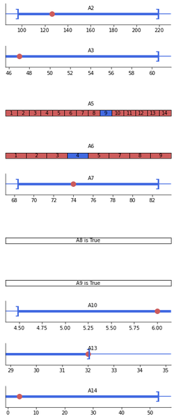
explainer.visualisation.notebook(instance, majoritary_reason)

---------   Theory Feature Types   -----------
Before the encoding (without one hot encoded features), we have:
Numerical features: 6
Categorical features: 4
Binary features: 4
Number of features: 14
Values of categorical features: {'A4_1': ['A4', 1, (1, 2, 3)], 'A4_2': ['A4', 2, (1, 2, 3)], 'A4_3': ['A4', 3, (1, 2, 3)], 'A5_1': ['A5', 1, (1, 2, 3, 4, 5, 6, 7, 8, 9, 10, 11, 12, 13, 14)], 'A5_2': ['A5', 2, (1, 2, 3, 4, 5, 6, 7, 8, 9, 10, 11, 12, 13, 14)], 'A5_3': ['A5', 3, (1, 2, 3, 4, 5, 6, 7, 8, 9, 10, 11, 12, 13, 14)], 'A5_4': ['A5', 4, (1, 2, 3, 4, 5, 6, 7, 8, 9, 10, 11, 12, 13, 14)], 'A5_5': ['A5', 5, (1, 2, 3, 4, 5, 6, 7, 8, 9, 10, 11, 12, 13, 14)], 'A5_6': ['A5', 6, (1, 2, 3, 4, 5, 6, 7, 8, 9, 10, 11, 12, 13, 14)], 'A5_7': ['A5', 7, (1, 2, 3, 4, 5, 6, 7, 8, 9, 10, 11, 12, 13, 14)], 'A5_8': ['A5', 8, (1, 2, 3, 4, 5, 6, 7, 8, 9, 10, 11, 12, 13, 14)], 'A5_9': ['A5', 9, (1, 2, 3, 4, 5, 6, 7, 8, 9, 10, 11, 12, 13, 14)], 'A5_10': ['A5', 10, (1, 2, 3, 4, 5, 6, 7, 8, 9, 10, 11, 12, 13, 14)], 'A5_11': ['A5', 11, (1, 2, 3, 4, 5, 6, 7, 8, 9, 10, 11, 12, 13, 14)], 'A5_12': ['A5', 12, (1, 2, 3, 4, 5, 6, 7, 8, 9, 10, 11, 12, 13, 14)], 'A5_13': ['A5', 13, (1, 2, 3, 4, 5, 6, 7, 8, 9, 10, 11, 12, 13, 14)], 'A5_14': ['A5', 14, (1, 2, 3, 4, 5, 6, 7, 8, 9, 10, 11, 12, 13, 14)], 'A6_1': ['A6', 1, (1, 2, 3, 4, 5, 7, 8, 9)], 'A6_2': ['A6', 2, (1, 2, 3, 4, 5, 7, 8, 9)], 'A6_3': ['A6', 3, (1, 2, 3, 4, 5, 7, 8, 9)], 'A6_4': ['A6', 4, (1, 2, 3, 4, 5, 7, 8, 9)], 'A6_5': ['A6', 5, (1, 2, 3, 4, 5, 7, 8, 9)], 'A6_7': ['A6', 7, (1, 2, 3, 4, 5, 7, 8, 9)], 'A6_8': ['A6', 8, (1, 2, 3, 4, 5, 7, 8, 9)], 'A6_9': ['A6', 9, (1, 2, 3, 4, 5, 7, 8, 9)], 'A12_1': ['A12', 1, (1, 2, 3)], 'A12_2': ['A12', 2, (1, 2, 3)], 'A12_3': ['A12', 3, (1, 2, 3)]}

Number of used features in the model (before the encoding): 14
Number of used features in the model (after the encoding): 38
----------------------------------------------
majoritary_reason 12

png

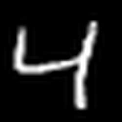
With an image dataset

We use a modified version of MNIST dataset that focuses on 4 and 9 digits. We create a model using the hold-out approach (by default, the test size is set to 30%). We choose to use a Boosted Tree by using XGBoost.

from pyxai import Learning, Explainer, Tools


# Machine learning part
learner = Learning.Xgboost("../dataset/mnist49.csv", learner_type=Learning.CLASSIFICATION)
model = learner.evaluate(method=Learning.HOLD_OUT, output=Learning.BT)
instance, prediction = learner.get_instances(model, n=1, correct=True, predictions=[0])

data:
       0  1  2  3  4  5  6  7  8  9  ...  775  776  777  778  779  780  781   
0      0  0  0  0  0  0  0  0  0  0  ...    0    0    0    0    0    0    0  \
1      0  0  0  0  0  0  0  0  0  0  ...    0    0    0    0    0    0    0   
2      0  0  0  0  0  0  0  0  0  0  ...    0    0    0    0    0    0    0   
3      0  0  0  0  0  0  0  0  0  0  ...    0    0    0    0    0    0    0   
4      0  0  0  0  0  0  0  0  0  0  ...    0    0    0    0    0    0    0   
...   .. .. .. .. .. .. .. .. .. ..  ...  ...  ...  ...  ...  ...  ...  ...   
13777  0  0  0  0  0  0  0  0  0  0  ...    0    0    0    0    0    0    0   
13778  0  0  0  0  0  0  0  0  0  0  ...    0    0    0    0    0    0    0   
13779  0  0  0  0  0  0  0  0  0  0  ...    0    0    0    0    0    0    0   
13780  0  0  0  0  0  0  0  0  0  0  ...    0    0    0    0    0    0    0   
13781  0  0  0  0  0  0  0  0  0  0  ...    0    0    0    0    0    0    0   

       782  783  784  
0        0    0    4  
1        0    0    9  
2        0    0    4  
3        0    0    9  
4        0    0    4  
...    ...  ...  ...  
13777    0    0    4  
13778    0    0    4  
13779    0    0    4  
13780    0    0    9  
13781    0    0    4  

[13782 rows x 785 columns]
--------------   Information   ---------------
Dataset name: ../dataset/mnist49.csv
nFeatures (nAttributes, with the labels): 785
nInstances (nObservations): 13782
nLabels: 2
---------------   Evaluation   ---------------
method: HoldOut
output: BT
learner_type: Classification
learner_options: {'seed': 0, 'max_depth': None, 'eval_metric': 'mlogloss'}
---------   Evaluation Information   ---------
For the evaluation number 0:
metrics:
   accuracy: 98.57315598548972
   precision: 98.53911404335533
   recall: 98.67862199150542
   f1_score: 98.60881867484083
   specificity: 98.4623015873016
   true_positive: 2091
   true_negative: 1985
   false_positive: 31
   false_negative: 28
   sklearn_confusion_matrix: [[1985, 31], [28, 2091]]
nTraining instances: 9647
nTest instances: 4135

---------------   Explainer   ----------------
For the evaluation number 0:
**Boosted Tree model**
NClasses: 2
nTrees: 100
nVariables: 1590

---------------   Instances   ----------------
number of instances selected: 1
----------------------------------------------

# Explanation part
explainer = Explainer.initialize(model, instance)
minimal_tree_specific_reason = explainer.minimal_tree_specific_reason(time_limit=10)
print("len minimal tree_specific_reason:", len(minimal_tree_specific_reason))

len minimal tree_specific_reason: 187

For a dataset containing images, you need to give certain information specific to images (through the image parameter of the show method) in order to display instances and explanations correctly. Here we give an example for the MNIST images, each of which is composed of 28 $\times$ 28 pixels, and the value of a pixel is an 8-bit integer:

import numpy

def get_pixel_value(instance, x, y, shape):
    index = x * shape[0] + y 
    return instance[index]

def instance_index_to_pixel_position(i, shape):
    return i // shape[0], i % shape[0]

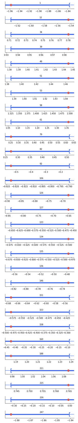
explainer.visualisation.notebook(instance, minimal_tree_specific_reason, image={"shape": (28,28),
                      "dtype": numpy.uint8,
                      "get_pixel_value": get_pixel_value,
                      "instance_index_to_pixel_position": instance_index_to_pixel_position})

png

<Figure size 432x288 with 0 Axes>

Blue (resp. Red) pixels represent positive (resp. negative) conditions in the explanation. A blue (resp. red) pixel means that the color of the pixel must be white (black) to be included in the explanation. In this way, all instances (images) that have white pixels when the explanation has blue pixels and have black pixels when the explanation has red pixels will have the same classification (in our case, it will be 4).

You can open on your screen the images with:

explainer.visualisation.screen(instance, minimal_tree_specific_reason, image={"shape": (28,28),
                      "dtype": numpy.uint8,
                      "get_pixel_value": get_pixel_value,
                      "instance_index_to_pixel_position": instance_index_to_pixel_position})

<Figure size 432x288 with 0 Axes>

You can save PNG files with:

explainer.visualisation.save_png("mnist49_example.png", instance, minimal_tree_specific_reason, image={"shape": (28,28),
                      "dtype": numpy.uint8,
                      "get_pixel_value": get_pixel_value,
                      "instance_index_to_pixel_position": instance_index_to_pixel_position})

<Figure size 432x288 with 0 Axes>

You can get PIL images with:

images = explainer.visualisation.get_PILImage(instance, minimal_tree_specific_reason, image={"shape": (28,28),
                      "dtype": numpy.uint8,
                      "get_pixel_value": get_pixel_value,
                      "instance_index_to_pixel_position": instance_index_to_pixel_position})
print(images)

[<PIL.Image.Image image mode=L size=28x28 at 0x7FF4D8850C10>, <PIL.Image.Image image mode=RGBA size=28x28 at 0x7FF4D86571F0>]

<Figure size 432x288 with 0 Axes>

You can resize a PIL image with:

image_resized = explainer.visualisation.resize_PILimage(images[1], 100)
from IPython.display import display
display(image_resized)

png

With a time series dataset

The ArrowHead dataset consists of outlines of the images of arrowheads. The shapes of the projectile points are converted into a time series using the angle-based method. The classes (called “Avonlea”, “Clovis” and “Mix”) are based on shape distinctions such as the presence and location of a notch in the arrow.

Note that we need the sktime package to load this dataset: python3 -m pip install sktime We start by preparing the data:

import pandas
from sktime.datasets import load_arrow_head

X, y = load_arrow_head()

rawdata = []
n_instances = X["dim_0"].shape[0]
n_features = len(X["dim_0"][0])
print("n_instances:", n_instances)
print("n_features:", n_features)

for i in range(n_instances):
    instance = X["dim_0"][i]
    label = y[i]
    rawdata.append(list(instance)+[label])
    
dataframe = pandas.DataFrame(rawdata)
dataframe.columns = [str(i) for i in range(n_features)]+["label"]
print(dataframe)
    

n_instances: 211
n_features: 251
            0         1         2         3         4         5         6   
 -1.963009 -1.957825 -1.956145 -1.938289 -1.896657 -1.869857 -1.838705  \
 -1.774571 -1.774036 -1.776586 -1.730749 -1.696268 -1.657377 -1.636227   
 -1.866021 -1.841991 -1.835025 -1.811902 -1.764390 -1.707687 -1.648280   
 -2.073758 -2.073301 -2.044607 -2.038346 -1.959043 -1.874494 -1.805619   
 -1.746255 -1.741263 -1.722741 -1.698640 -1.677223 -1.630356 -1.579440   
..        ...       ...       ...       ...       ...       ...       ...   
-1.625142 -1.622988 -1.626062 -1.610799 -1.568567 -1.552384 -1.535922   
-1.657757 -1.664673 -1.632645 -1.611002 -1.591838 -1.548710 -1.502004   
-1.603279 -1.587365 -1.577407 -1.556043 -1.531201 -1.505051 -1.487764   
-1.739020 -1.741534 -1.732863 -1.722299 -1.698109 -1.665590 -1.618474   
-1.630727 -1.629918 -1.620556 -1.607832 -1.579719 -1.562561 -1.526980   

            7         8         9  ...       242       243       244   
 -1.812289 -1.736433 -1.673329  ... -1.655329 -1.719153 -1.750881  \
 -1.609807 -1.543439 -1.486174  ... -1.484666 -1.539972 -1.590150   
 -1.582643 -1.531502 -1.493609  ... -1.652337 -1.684565 -1.743972   
 -1.731043 -1.712653 -1.628022  ... -1.743732 -1.819801 -1.858136   
 -1.551225 -1.473980 -1.459377  ... -1.607101 -1.635137 -1.686346   
..        ...       ...       ...  ...       ...       ...       ...   
-1.498036 -1.460416 -1.430095  ... -1.447404 -1.476224 -1.531105   
-1.447861 -1.389342 -1.322178  ... -1.580908 -1.631919 -1.664673   
-1.455712 -1.419410 -1.391145  ... -1.492721 -1.511071 -1.539271   
-1.585797 -1.547740 -1.504280  ... -1.487935 -1.536131 -1.594358   
-1.507067 -1.464752 -1.417547  ... -1.350127 -1.403990 -1.451258   

          245       246       247       248       249       250  label  
 -1.796273 -1.841345 -1.884289 -1.905393 -1.923905 -1.909153      0  
 -1.635663 -1.639989 -1.678683 -1.729227 -1.775670 -1.789324      1  
 -1.799117 -1.829069 -1.875828 -1.862512 -1.863368 -1.846493      2  
 -1.886146 -1.951247 -2.012927 -2.026963 -2.073405 -2.075292      0  
 -1.691274 -1.716886 -1.740726 -1.743442 -1.762729 -1.763428      1  
..        ...       ...       ...       ...       ...       ...    ...  
-1.551077 -1.567998 -1.597641 -1.623653 -1.622988 -1.624174      2  
-1.672895 -1.678613 -1.666825 -1.667466 -1.681769 -1.678613      2  
-1.565389 -1.577493 -1.585284 -1.603086 -1.605382 -1.605597      2  
-1.615147 -1.636495 -1.669889 -1.699870 -1.713118 -1.728176      2  
-1.472321 -1.513637 -1.550431 -1.581576 -1.595273 -1.620783      2  

[211 rows x 252 columns]

We create a model using the hold-out approach (by default, the test size is set to 30%). We choose to use a Boosted Tree by using XGBoost.

from pyxai import Learning, Explainer, Tools


# Machine learning part
learner = Learning.Xgboost(dataframe, learner_type=Learning.CLASSIFICATION)
model = learner.evaluate(method=Learning.HOLD_OUT, output=Learning.BT)
instance, prediction = learner.get_instances(model, n=1, correct=True, predictions=[0])

data:
            0         1         2         3         4         5         6   
0   -1.963009 -1.957825 -1.956145 -1.938289 -1.896657 -1.869857 -1.838705  \
1   -1.774571 -1.774036 -1.776586 -1.730749 -1.696268 -1.657377 -1.636227   
2   -1.866021 -1.841991 -1.835025 -1.811902 -1.764390 -1.707687 -1.648280   
3   -2.073758 -2.073301 -2.044607 -2.038346 -1.959043 -1.874494 -1.805619   
4   -1.746255 -1.741263 -1.722741 -1.698640 -1.677223 -1.630356 -1.579440   
..        ...       ...       ...       ...       ...       ...       ...   
206 -1.625142 -1.622988 -1.626062 -1.610799 -1.568567 -1.552384 -1.535922   
207 -1.657757 -1.664673 -1.632645 -1.611002 -1.591838 -1.548710 -1.502004   
208 -1.603279 -1.587365 -1.577407 -1.556043 -1.531201 -1.505051 -1.487764   
209 -1.739020 -1.741534 -1.732863 -1.722299 -1.698109 -1.665590 -1.618474   
210 -1.630727 -1.629918 -1.620556 -1.607832 -1.579719 -1.562561 -1.526980   

            7         8         9  ...       242       243       244   
0   -1.812289 -1.736433 -1.673329  ... -1.655329 -1.719153 -1.750881  \
1   -1.609807 -1.543439 -1.486174  ... -1.484666 -1.539972 -1.590150   
2   -1.582643 -1.531502 -1.493609  ... -1.652337 -1.684565 -1.743972   
3   -1.731043 -1.712653 -1.628022  ... -1.743732 -1.819801 -1.858136   
4   -1.551225 -1.473980 -1.459377  ... -1.607101 -1.635137 -1.686346   
..        ...       ...       ...  ...       ...       ...       ...   
206 -1.498036 -1.460416 -1.430095  ... -1.447404 -1.476224 -1.531105   
207 -1.447861 -1.389342 -1.322178  ... -1.580908 -1.631919 -1.664673   
208 -1.455712 -1.419410 -1.391145  ... -1.492721 -1.511071 -1.539271   
209 -1.585797 -1.547740 -1.504280  ... -1.487935 -1.536131 -1.594358   
210 -1.507067 -1.464752 -1.417547  ... -1.350127 -1.403990 -1.451258   

          245       246       247       248       249       250  label  
0   -1.796273 -1.841345 -1.884289 -1.905393 -1.923905 -1.909153      0  
1   -1.635663 -1.639989 -1.678683 -1.729227 -1.775670 -1.789324      1  
2   -1.799117 -1.829069 -1.875828 -1.862512 -1.863368 -1.846493      2  
3   -1.886146 -1.951247 -2.012927 -2.026963 -2.073405 -2.075292      0  
4   -1.691274 -1.716886 -1.740726 -1.743442 -1.762729 -1.763428      1  
..        ...       ...       ...       ...       ...       ...    ...  
206 -1.551077 -1.567998 -1.597641 -1.623653 -1.622988 -1.624174      2  
207 -1.672895 -1.678613 -1.666825 -1.667466 -1.681769 -1.678613      2  
208 -1.565389 -1.577493 -1.585284 -1.603086 -1.605382 -1.605597      2  
209 -1.615147 -1.636495 -1.669889 -1.699870 -1.713118 -1.728176      2  
210 -1.472321 -1.513637 -1.550431 -1.581576 -1.595273 -1.620783      2  

[211 rows x 252 columns]
--------------   Information   ---------------
Dataset name: pandas.core.frame.DataFrame
nFeatures (nAttributes, with the labels): 252
nInstances (nObservations): 211
nLabels: 3
---------------   Evaluation   ---------------
method: HoldOut
output: BT
learner_type: Classification
learner_options: {'seed': 0, 'max_depth': None, 'eval_metric': 'mlogloss'}
---------   Evaluation Information   ---------
For the evaluation number 0:
metrics:
   micro_averaging_accuracy: 89.58333333333334
   micro_averaging_precision: 84.375
   micro_averaging_recall: 84.375
   macro_averaging_accuracy: 89.58333333333334
   macro_averaging_precision: 84.61147421931736
   macro_averaging_recall: 85.05072463768116
   true_positives: {'0': 18, '1': 22, '2': 14}
   true_negatives: {'0': 37, '1': 36, '2': 45}
   false_positives: {'0': 2, '1': 5, '2': 3}
   false_negatives: {'0': 7, '1': 1, '2': 2}
   accuracy: 84.375
   sklearn_confusion_matrix: [[18, 4, 3], [1, 22, 0], [1, 1, 14]]
nTraining instances: 147
nTest instances: 64

---------------   Explainer   ----------------
For the evaluation number 0:
**Boosted Tree model**
NClasses: 3
nTrees: 300
nVariables: 345

---------------   Instances   ----------------
number of instances selected: 1
----------------------------------------------

Next, we calculate an explanation for an arrow (an instance) that is classified as 0 (corresponding to the Avonlea era). We have fix the time limit to 60 seconds, but we obtain the same result with 10 seconds.

# Explanation part
explainer = Explainer.initialize(model, instance)
tree_specific_reason = explainer.tree_specific_reason(time_limit=60)
print("tree_specific_reason:", len(tree_specific_reason))

tree_specific_reason: 38

If we display in a Jupyter notebook this explanation, it is difficult to interpret.

explainer.visualisation.notebook(instance, tree_specific_reason)

png

To overcome this problem, we display it as a time series.

explainer.visualisation.notebook(instance, tree_specific_reason, time_series={"serie":learner.feature_names[:-1]}, width=600)

png

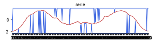
The red line represents the instance values. The two blue lines represent the extreme values of the explanation for each feature. A blue value at the top (resp. at the bottom) means that the extreme value for the associated feature is $+\infty$ (resp. $-\infty$).

The explanation shows us that all the other instances (other lines we can imagine) between the two blue lines will have the same classification. In our case, we clearly see that the explanation tells us that it is because of the two bumps on each side that this instance is classified as such.